Selection of Image Sub-area for Image Registration:
Registration and Cross Section Alignment Tool
David Clutter, Sang-Chul Lee and Peter Bajcsy
Introduction
This tool is designed to support researchers in making registration decisions about image size to be used for alignment (registration). In our application scenario, a researcher would like to align a pair of image stacks that were acquired by a fluorescent confocal laser scanning microscope (CLSM). There might be an image sub-area of a specific importance although the surrounding of the sub-area is also of a potential interest (see Figure 1). One would like to understand the tradeoffs between accuracy of alignment and the image size to be used for alignment.
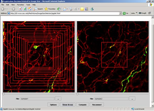
Figure 1. Illustration of the registration decision about image sub-area size. A similarity of a pair of sub-areas from the left and right images is assessed by computing a normalized correlation value that depends on area selection and its size.
We provide a tool for:
- loading two registered images, e.g., from one CLSM stack,
- selecting a sub-area of interest, and
- computing the goodness of match measured by normalized correlation for increasing sub-area size.
In general, this type of data-driven analysis allows a researcher to understand the tradeoffs between image size and the expected alignment accuracy when the task is to align two unregistered images, e.g., from two spatially adjacent CLSM stacks. One can then make an optimal registration decision about image size so that the alignment result is a compromise between spatial image size and alignment accuracy. It is also possible to perform studies for two unregistered images by searching a range of possible translations, rotations, scales and shears (affine transformation model). In this case, the tool will report the maximum correlation value for each sub-area.
Instructions
First, click START to launch the tool in a new window
You should see a Warning – Security dialog shown in Figure 2. Click the Yes button to proceed. A new window will appear with two preloaded CLSM images containing two red and green bands (see Figure 3)
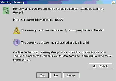
Figure 2: Security warning dialog. Please, click Yes to proceed.
Second, you might load your own images in File. The loading might take some time depending on your image size and bandwidth connection.
Third, with a left mouse button, click and drag the mouse to define an area of the highest importance. You can click the Show Area button at the bottom of the window to see all sub-areas that would be explored. The result of this operation is illustrated in Figure 1. If you would like to change the scale factor of sub-area increments, click the button Options. A new dialog will appear (see Figure 4). One can set the scale factor of sub-area increments by moving the slider bar under Scale Factor. The value will be applied to width and height of the selected rectangular sub-area as the percentage of its increase. The computation is described as:
new height=height*(1+ScaleFactor/100)
and
new width=width*(1+ScaleFactor/100).
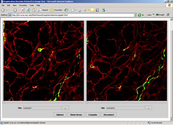
Figure 3: Initial window with the preloaded sample images.
The slider bar under “Radius” refers to the input parameter for two unregistered images. Normalized correlation values are computed over multiple spatial alignment configurations of two input images, where the configurations are obtained by affine transformation of the right image and a copy of the left image. The affine transformation parameters are derived from triplets of pixels that (a) are located near three corners of a sub-area, and (b) come from the neighborhood of (2*Radius+1)x(2*Radius+1) of these three pixels.
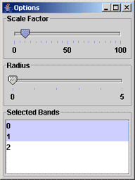
Figure 4: The dialog labeled as Options is for setting (1) a scale factor of the selected sub-area growth, (2) a radius for alignment optimization of two unregistered images, and (3) selected bands that would be evaluated.
The Options dialog also provides an interface to define which bands should be processed since the correlation values are computed per band. A band can be selected by left mouse button click on the band index in the area labeled as Selected Bands. Multiple bands can be selected by holding Ctrl key while using the left mouse button clicks.
After options have been specified, one can launch the computation by clicking on the Compute button in the main frame (shown in Figure 3). A new job window shown in Figure 5 will appear and report information about the job identification number (Job ID), submitted date/time, start date/time of execution and finish date/time of execution, and the current job status. These pieces of information can be seen in Figure 5, top. A job can be aborted by clicking on the Abort button. The job window can be closed by clicking on the Done button with or without aborting the job since the job might take several hours. If a job runs for a long period of time, then one would remember the Job ID and recover the results of computation by (a) returning to the main web page later in time, and (b) reconnecting to the job by clicking on the Reconnect button in the main window (shown in Figure 3).
Once the computation has been completed, the View Result button in the job window (Figure 5, bottom) is provided for viewing the results. The results are presented either as a graph if the Result tab is selected or as a text if the Log tab is selected by mouse clicking it. Examples of a graph output and a text output are presented in Figure 5 (graph) and Figure 6
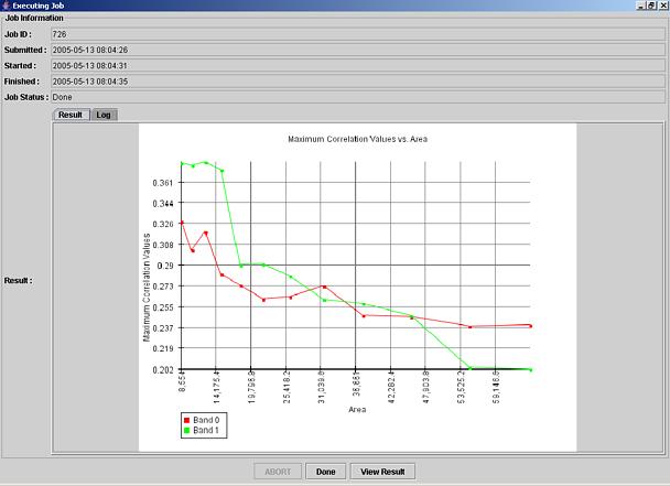
Figure 5: The resulting graph with maximum normalized correlation values as a function of sub-area size.
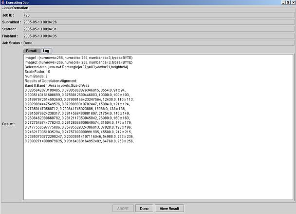
Figure 6: An example of a text output with parameters (Scale factor, number of bands and image information) and maximum normalized correlation values per band as a function of sub-area size (area defined in pixels and defined as number of rows x number of columns).
Image Manipulation
Additional image manipulation and navigation operations are available. In order to change zoom level, set gamma correction, or select displayed image bands, one should right mouse button click over an image panel and the menu will appear for selection (see Figure 7). These options are explained next.
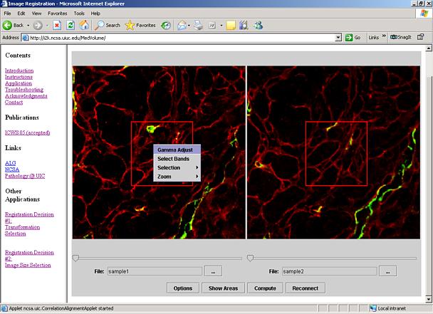
Figure 7: Image manipulation menu is shown when the left mouse button is clicked over one of the image panels.
Image Zoom: changes digital resolution of an image. The option Fit will automatically rescale an image to fit the image panel size. The option Custom lets a user define the scaling factor either as a multiplicative factor or as a percentage (by appending % to the number) of the original image size. For example using the number 2, or 200% will result in an image that is twice the size of the original.
Gamma: The dialog Select Gamma appears after right mouse button click and selection of the Gamma option. The dialog slider bar and the edit box are for setting the image brightness (gamma factor).
Select Bands: The dialog Select Bands shown in Figure 7 appears after right mouse button click and selection of the Select Bands option. The dialog slider bars and edit boxes provide a way to choose which input image band will be displayed in which color band (red, green or blue color bands). If a grayscale mode is preferred then the check box Use Grayscale should be checked and the slider bar below it defines the displayed band. The button Apply is for executing the desired band assignment. The preview window above the band assignment entries is designed to show a preview of the resulting image.
When the image panels are in the gray scale mode then the slider bar in the main window is enabled and one can select with the slider any single band for viewing. An example of this case is shown in Figure 8.
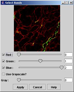
Figure 8: Select bands dialog.
Image navigation:
If the spatial area of a displayed image is larger than the allocated window then the image will appear in a scroll panel. The navigation is enabled with sliding horizontal and vertical scroll bars to view any area of interest.
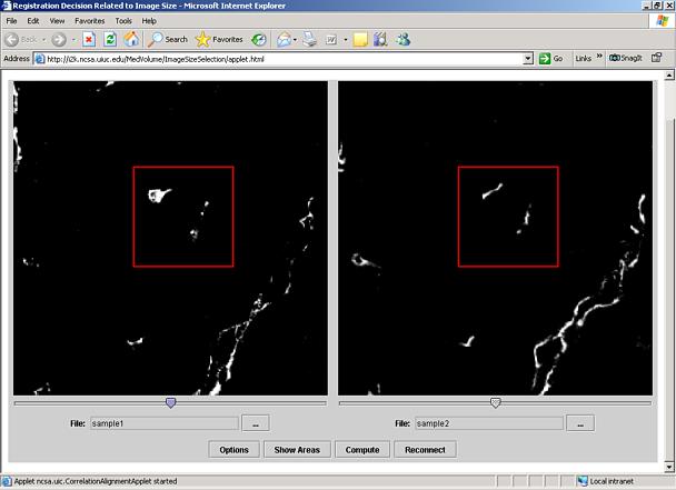
Figure 9: An example of the use of the slider bar under the image panels in the gray scale mode. The images correspond to the green bands of the test data uploaded automatically when the tool is launched.
Additional Notes
- Identical Images:
If two identical frames would be compared then their normalized correlation value should be equal to one. However, we have not seen identical frames in the case of repetitive fluorescent imaging and hence we default the normalized correlation value for this specific case to zero.
- Interpretation of normalized correlation values:
In general, the higher the normalized correlation value, the better image match.
- Range of normalized correlation values:
The range of normalized correlation values is [0, 1].
- Band interpretation:
When one would like to process only a subset of bands present in two color images then the band to color correspondence is as follows, band 0 ~ red, band 1 ~ green, and band 2 ~ blue.
Examples
- Alignment Tool 1 - Cross sections of blood vessels.
- Alignment Tool 2 - Image Size Selection.


